Quickstart

Once you have installed mbb, import it in a python script:

from mbb import ModifiedBlackbody as MBB

The first step is usually to create a MBB model by filling in the necessary initial parameters:

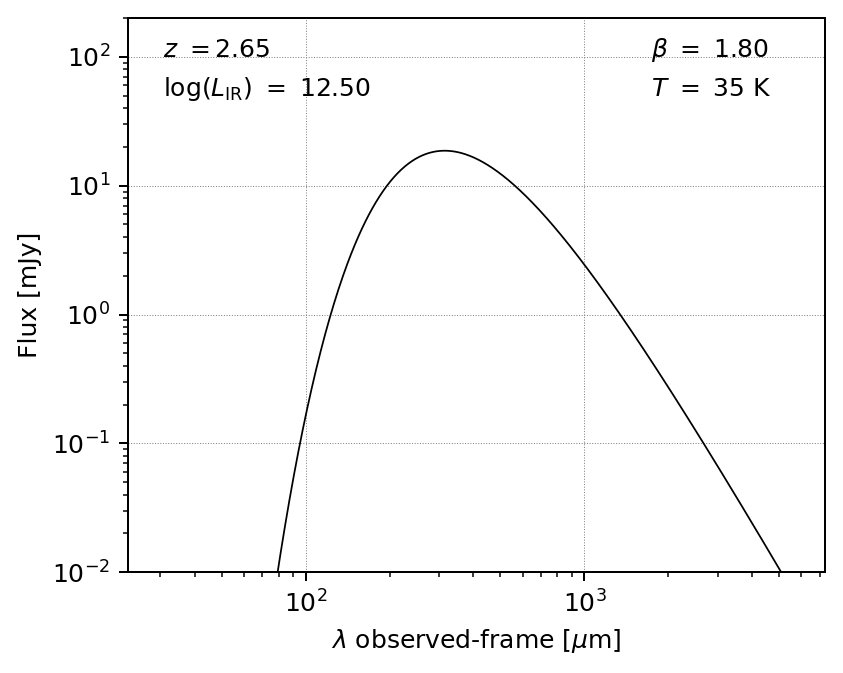
m = MBB(L=12.5, T=35, beta=1.8, z=2.65, opthin=True, pl=False)

Here we have chosen an optically thin model with no mid-infrared power law. A quick plot of this model can be made, if desired:

import matplotlib.pyplot as plt

fig, ax = m.plot_sed(obs_frame=True)
plt.show()

Alternatively, we could choose, say, a general opacity model with the power law included (default power-law slope alpha=2.0 and turnover wavelength l0=200 microns):

m2 = MBB(L=12.5, T=35, beta=1.8, z=2.65, opthin=False, pl=True)
fig, ax = m2.plot_sed(obs_frame=True)
plt.show()

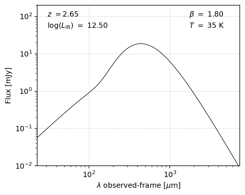
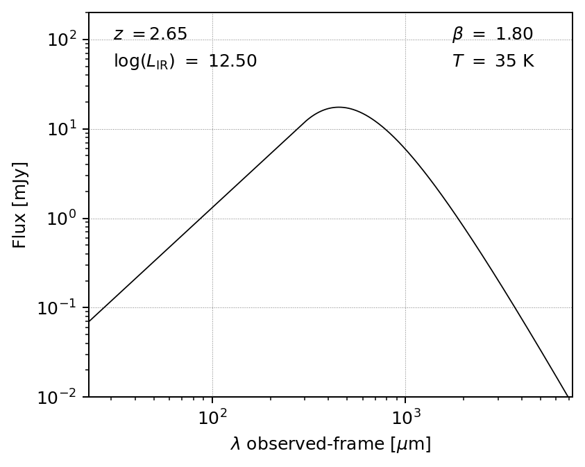
The above model follows Casey (2012), where the power law is joined at 3/4 the wavelength where the slope equals alpha. If you prefer a piecewise power law connected where the slope of the blackbody matches alpha, set pl_piecewise to True:

m3 = MBB(L=12.5, T=35, beta=1.8, z=2.65, opthin=False, pl=True, pl_piecewise=True)
fig, ax = m3.plot_sed(obs_frame=True)
plt.show()

Fitting photometric data

Most often, you want to fit a given model to photometric data points. mbb allows for Bayesian model fitting via the fit() method, which uses the emcee package to perform Markov Chain Monte Carlo (MCMC) sampling of the parameter space.

The phot keyword should be a 3 x N array (wavelengths in microns, fluxes in Jy, and errors in Jy). Pass restframe=True if the wavelengths are in the rest frame, otherwise it will default to observed frame. This photometry is stored in the phot attribute of the MBB instance (observed frame) and the phot_rf attribute (rest frame). (note: internally all photometry is converted to rest frame).

Note: mbb handles upper limits correctly in the Bayesian likelihood function. To specify which data should be treated as upper limits, pass a boolean array to the uplims keyword of fit(). The code assumes that, for each photometric band labeled as an upper limit, the flux value should be used as the limit (accounting for the \(1\sigma\) uncertainty as well) if it is positive and larger than the \(1\sigma\) error, otherwise this error is used as the limit.

import numpy as np
phot = np.array(
        [[250, 350, 450, 850, 1200], # wavelength in microns
         [0.012, 0.019, 0.0166, 0.00683, 0.0023], # flux in Jy
         [0.0044, 0.0064, 0.0036, 0.00057, 0.0003]]  # error in Jy
        )
    uplims=phot[1]/phot[2] < 3.0 # upper limit if not detected at >= 3-sigma
    result = m.fit(phot=phot, uplims=uplims, niter=1000, params=['L', 'T', 'beta'])

Running burn-in...
100%|█████████████████████████████████████| 1000/1000 [00:35<00:00, 27.80it/s]
Running fitter...
100%|█████████████████████████████████████| 1000/1000 [00:37<00:00, 26.34it/s]
Done

You specify which parameters to fit using the params keyword argument; the options are L, T, beta, alpha, l0, or z (the latter if you want to use mbb as a far-infrared photometric redshift code). The parameter values used to initialize the ModifiedBlackbody are also used by emcee as the starting parameters of the fit.

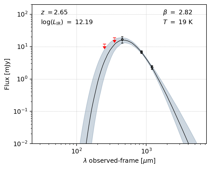
View the resulting model after the fit, with uncertainties:

fig, ax = m.plot_sed(obs_frame=True)
plt.show()

You can also make a simple corner plot of the parameters that were varied:

fig = m.plot_corner()
plt.show()

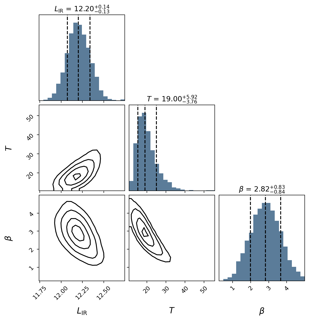
The basic plotting routines are fairly sparse, but most plot aspects can be modified, or you can write your own functions to produce higher quality / publication-ready figures.

Modeling priors

By default, uniform priors are assumed on all the fit parameters, but you can change this by passing a dictionary, priors, to fit. Each key of priors should be the name of a parameter, and each value is either:

1. a dictionary with keywords mu and sigma, to specify Gaussian priors

2. your own function, which takes the parameter as an argument and returns the probability density of that parameter value.

result = m.fit(phot=phot, niter=1000, params=['L', 'T', 'beta'],
    restframe=False, priors = {'beta':dict(mu=1.8,sigma=0.3)})

Running burn-in...
100%|█████████████████████████████████████| 1000/1000 [00:36<00:00, 27.32it/s]
Running fitter...
100%|█████████████████████████████████████| 1000/1000 [00:36<00:00, 27.20it/s]
Done

Accessing the fit results

To access the percentiles of the posterior distribution for any parameter in the fit:

print(m.post_percentile('beta', q=(16,50,84))) #16th, 50th, 84th percentiles

[1.63739978 1.90546219 2.17945187]

To get the reduced chi-squared value from the fit_result:

reduc_chi2 = m.fit_result['chi2'] / (m.fit_result['n_bands']-m.fit_result['n_params'])
print(chi2)

0.8526608373363864

Currently, the measurement for L requires integration under the hood, so it can take a long time. The same applies for generating the corner plots. I’m working on speeding this process up.

The full emcee.EnsembleSampler is stored as the sampler element of the fit_result dictionary. This can be used to perform any kind of analysis one would typically want with emcee, such as looking at the autocorrelation time and other fit statistics, if desired.

To clear the fit_result and priors, use reset(). Note that the parameters of the MBB will still be set to the best values from the previous fit:

m.reset()
print(np.round(m.beta,2))

1.91

Other utility functions

The ModifiedBlackbody class also includes a few helper functions and attributes to compute useful quantities, such as fluxes, luminosities, and dust masses:

Flux at a given wavelength:

To get the model flux at a given wavelength, pass a value or array of wavelengths (in micron) to eval(). By default, this assumes observed-frame wavelengths, but you can specify a rest-frame wavelength by passing z = 0 (i.e., shifting the observed SED to \(z = 0\)).

m.eval(1200) #wl in microns, observed frame by default

0.0024958420867594506 Jy

import astropy.units as u

np.round(m.eval(100, z=0).to(u.mJy), 3) #rest frame 100um

18.438 mJy

Infrared luminosity:

print(m.get_luminosity(wllimits=(8,1000))) #8-1000um gives same luminosity as m.L. Can choose any rest frame wavelength limits desired.
print(np.round(np.log10(m.get_luminosity(wllimits=(8,1000)).value),2))
print(np.round(m.L,2))

2499320878862.3975 solLum
12.40
12.40

Dust mass:

np.log10(m.dust_mass.value) #solMass

8.804948529939795

Wavelength where dust emission peaks (proxy for temperature):

m.get_peak_wavelength() # note this is a rest-frame wl

108.2946298908265 micron

Multiprocessing

By default, mbb will try to use the number of available CPUs minus 2 to run the fit. To control this, you can either pass an integer to the ncores argument of fit (pass 1 to not use multiprocessing at all), or you can generate your own process Pool object (e.g., multiprocessing.pool.Pool) and pass it as the pool argument.

Note: to avoid multiprocessing errors, the process start method is set to “fork” on Linux/macOS and to “spawn” on Windows. If you run into errors, I recommend passing in your own Pool object or forgoing multiprocessing.